Recently I dug a bit into sound classification and during some research I wanted to understand a bit more about networks that learn their objective end-to-end. End-to-end in this context means there is no feature engineering. The network learns it’s own features in certain layers.
Basics
There are two main types of features when working with sound data in ML. Either
spectograms or the raw data (normalized to a numerical range \( s=\{-1, 1\} \)).
Here is an example using torchaudio,
which automatically loads values in this range. Other implementations like
librosa do the same.
from torchaudio.utils import download_asset


sample = download_asset(
    "tutorial-assets/Lab41-SRI-VOiCES-src-sp0307-ch127535-sg0042.wav"
)
signal, sample_rate = torchaudio.load(sample)
print(signal.size())
# torch.Size([1, 54400])
print(signal.min(), signal.max())
Feautre extraction
The goal of end-to-end soundclassification is to provide a way to extract features directly from the raw audio samples and learn them deeper down the line. In other words, there’s a feature extraction and a classification mechanism in the same network.
If we’d use spectograms we design a feature by applying Fourier Transformations along the time domain of the signal and obtain a frequency spectrum of that time domain. A spectogram like a Mel Spectogram uses these frequency spectrum by splitting the time domain into windows and sample the frequency spectrum over the windows (and a hop length) and create a new time domain where each time step is corresponding to a frequency range scale - a mel scale.
Learning features
Since an end-to-end sound classification network does not extract features beforehand, but extracts these on-the-fly, we don’t need to do that. In machine learning many applications including computer vision use convolutions to extract features from a signal (or images for that matter).
To illustrate how this works, I use the work of Tokozume et.al., as their work is very
well know and cited in academica. Their publication is available in
Learning Environmental Sounds with End-to-End Convolutional Neural Networks.
They propose a system called EnvNet that is trained on
ESC-50, for environmental sound classification
(ESC). In order to understand their work better and play a little with it, I implemented
their work with PyTorch. This and some other related models can be
found in my esc-learner repo.
EnvNet looks like this:
class EnvNet(Module):
    def __init__(self, num_classes: int):
        super(EnvNet, self).__init__()
        self.num_classes = num_classes
        self.feature_conv = Sequential(
            OrderedDict(
                [
                    ("conv1", ConvBlock(1, 40, (1, 8))),
                    ("conv2", ConvBlock(40, 40, (1, 8))),
                    ("pool2", MaxPool2d((1, 160))),
                    ("transpose", Transpose(1, 2)),
                ]
            )
        )
        self.classifier = Sequential(
            OrderedDict(
                [
                    ("conv3", ConvBlock(1, 50, (8, 13))),
                    ("pool3", MaxPool2d(3)),
                    ("conv4", ConvBlock(50, 50, (1, 5))),
                    ("pool4", MaxPool2d((1, 3))),
                    ("flatten", Flatten(1, -1)),
                    ("fc5", LinearBlock(50 * 11 * 14, 4096)),
                    ("fc6", LinearBlock(4096, 4096)),
                    ("fc7", Linear(4096, self.num_classes)),
                ]
            )
        )
The part we are interested for now is self.feature_conv. This sequential part is
responsible for learning features. It uses two 2d Convolution blocks, where each block has
a few Submodules. Each block consist of a Conv2d, BatchNorm2d and a ReLU activation.
Further I want to explore a little what happens in this part of the network.
Here is the rest of it:
class ConvBlock(Module):
    def __init__(
        self, in_channels: int, out_channels: int, kernel_size: Union[int, tuple]
    ):
        super(ConvBlock, self).__init__()
        self.module = Sequential(
            Conv2d(in_channels, out_channels, kernel_size, bias=False),
            BatchNorm2d(out_channels),
            ReLU(),
        )

    def forward(self, X: Tensor) -> Tensor:
        return self.module(X)


class Transpose(Module):
    def __init__(self, target: int, destination: int):
        super(Transpose, self).__init__()
        self.target = target
        self.destination = destination

    def forward(self, X: Tensor) -> Tensor:
        return X.transpose(self.target, self.destination)


class LinearBlock(Module):
    def __init__(self, in_features: int, out_features: int):
        super(LinearBlock, self).__init__()
        self.module = Sequential(
            Linear(in_features, out_features),
            ReLU(),
            Dropout(),
        )

    def forward(self, X: Tensor) -> Tensor:
        return self.module(X)
The Transpose-Layer is jsut a wrapper around torch.transpose, to swap axis. And each
LinearBlock-Layer holds the same activation function ReLU (Rectangular Linear Unit)
as the ConvBlock.
Convolution
A convolutional layer holds a set of learnable filters. These filters all have a width and
a height. Depending on it’s kind dimension your convolutional layer has more parameters in
the filters. A Conv2d has a width and a hight. A Conv3d has an addionally parameter
which comes in handy when working with images. E.g. (5, 5, 3) would be correspond to
(h, w, c) (height, width and rgb-channels). These layers always provide an input and an
output dimension. The output dimension is also refered to as the number of filters.
Each filter will learn to focus on a different characteristic in the input data during
training. Another hyperparameter is stide. With strides we define something like a step
size for the filter. With stide=3, the filter will not sample every value in the
corresponding axis, but moves along the axis with step size 3. Lastly with padding we can
control if the output should pad to a certain length (for each dimension differently if
needed), which can be usefull if we want to preserve a certain length in any dimension.
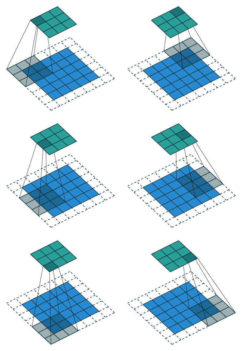
Convolution Arithmetic has a really nice gif illustrations of how the different hyperparameters of convolutions work. Here is an example where the blue map is the input, and cyan map is the output.

In this example we see a padded convolution (meaning the input is padded by 1 in each dim at start and end) with a (3, 3) kernel and a stride of (2, 2), meaning the kernel is moving 2 elements in both width and height over the input.
For each output dimension of this convolution a weight is learned. So if a convolution would except 1 input dimension and outputs 32, 32 of these weights are learned by looking at same region but activate on different types of inputs. It’s easier to understand this layer if we inspect it a little:
# A convolution of 1 input dims and 32 output dims, with
# padding of 1 in both dimensions and a stride of 2 in both
# dimensions of the convolution.
c = Conv2d(1, 32, 3, padding=(1, 1), stride=(2, 2))
x = torch.rand(4, 1, 5, 5)
print(c(x).shape)
# torch.Size([4, 32, 3, 3])
print(c.weight.size())
# torch.Size([32, 1, 3, 3])
As the example shows we obtain a matrix of shape (4, 32, 3, 3), since the batch_size
N=4, output / number of filters F=32 and the input dimensions of (5, 5), padded by 1
and strided by 2 shaped it to these sizes, just like in the figure shown above.
Feature extraction with convolutional layers
Going back to the network in Learning features. The authors
(Tokozume et.al.) of EnvNet propose a feature extraction block with two convolution blocks
where each constist of a Conv2d a BatchNorm2d and a ReLU activation function plus
a MaxPool2d layer. They work with a sample rate of 16 kHz and perform best when working
with samples 1.5 seconds long. So the input sample should contain 24000 samples.
Since the strides shown in the convolutions of the above section would sample odd output
shapes they add additional 14 samples, totaling 24014 samples per input.
Here’s a small demo:
def overlapping_samples_post_conv(num_sample: int, filter_size: int) -> int:
    return num_sample // (num_sample // filter_size) - 1


# Batch size N, audio channels, sample rate, number of classes, seconds per sample
N, channels, S, C, sec_per_sample = (1, 1, 16000, 50, 1.5)
# Find the number of samples to additionally take from the sample, so the convolution
# strides to even length (multiply by 2 since we have the same stride two times).
pad_samples = overlapping_samples_post_conv(S, 8) * 2
sample_size = int(np.floor(S * sec_per_sample + pad_samples))
# Simulated sound with the configured sample size
inputs = torch.rand(N, channels, sample_size)
# Unsqueeze so it fits into Conv2d
inputs = inputs.unsqueeze(1)

feature_conv = Sequential(
    ConvBlock(1, 40, (1, 8)),
    ConvBlock(40, 40, (1, 8)),
    MaxPool2d((1, 160)),
    Transpose(1, 2),
)

for module in feature_conv:
    print(module.__class__.__name__)
    inputs = module(inputs)
    print(inputs.size())

# ConvBlock
# torch.Size([1, 40, 1, 24007])
# ConvBlock
# torch.Size([1, 40, 1, 24000])
# MaxPool2d
# torch.Size([1, 40, 1, 150])
# Transpose
# torch.Size([1, 1, 40, 150])
We can see we output a batch with shape (1, 1, 40, 150). We still have the 40 dimensions
we propagated through 2 ConvBlocks whereas the time domain has reduced to 150.
We can now view each convoluted dimension as mel and each of the last 150 dimensions as a
time step, which gives us the diagram structure of a mel spectrogram if we manage to
inspect the frequency response.
We can observe how the convolution behaves when we train with actual data and for each
batch perform a back propagation, to classifiy environmental classes for these sounds.
To test the outputs of the FeatureConvolution module one can generate a sin curve for
different frequencies and input them after each training step. We now average each
dimension of the convolution along the time domain (in the outputs shape 150, the last
dim).

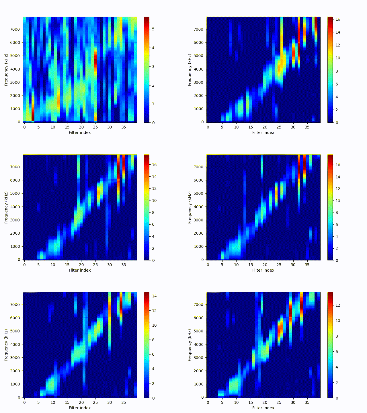
Frequency response (10-8000 Hz) of feature convolution filters (40) during training sorted by the average centered response. Gif shows one frame per epoch over 150 epochs. Filters are initialized randomly.
Originally the filters are not sorted. So the index is not the correct number internally, but shows the relation show to mel spectrograms. We can see that the learned filters handle the data pretty well, each filter responds to a certain range of frequency domain.
PS: For a few more end-to-end architectures for environmental sound classification have a look at esc-learner.